Predicting delivery time in volatile operational scenarios

At 1mg, improving customer experience at every touchpoint is of utmost importance. One of them is providing customers a seamless order delivery experience and a realistic view of the date and time of delivery. An accurate ETA (Estimated Time of Arrival) not only leads to a better customer experience but also reduces the unnecessary load on the customer care team. However, predicting the accurate delivery date or time is tricky and complex as few situations are inherently unpredictable.In our previous article, we talked about how we structured the problem of predicting ETA and the basics of our model. In this article, we will talk about the challenges we faced and how we upgraded our model to predict ETA in case of volatile demand. Starting from a relatively fluctuating performance, we achieved a stable high level of accuracy for our predictions spanning across months.

ETA 101

Before we start, here is a brief intro to the terminology we use. For a detailed understanding of the basics, please read the previous article in the series.

1. ETA: Estimated Time of Arrival of an order
2. Accuracy, breach and early delivery: This is the key metric we use for measuring our ETA prediction performance. If an order gets delivered within the promised time, the prediction is accurate. In case it is delivered beyond the last promised date, it is considered a breach. if the delivery happens before the first promised date, it is early delivery.
3. ETA bucket and bucket size: ETA bucket refers to the interval of ETA, e.g., 25th to 27th March. Bucket size refers to the length of the ETA bucket, e.g., 25th to 27th March is a 2-day window (can be classified as a 3-day window based on the nomenclature).

Maintaining ETA accuracy: A game of Whack-A-Mole

In our experience, maintaining a level of accuracy in ETA predictions was a game of whack-a-mole. At a point in time, we would face high percentage of orders getting breached and try to fix it through conservative ETA predictions. By the time we took an action, the operational situation would change entirely and the predicted ETAs would be longer than the actual delivery date. This cycle repeated itself and we found ourselves in an endless loop of whacks.The main reason for this was that while observing the performance of a model in production, we were looking at the consequences of things a few days back because of time taken to deliver the orders. For eg: If a warehouse was processing orders at a slower pace on a particular day, the impact on ETA accuracy is visible only post delivery (or ETA breach) of the orders placed on that day. This creates a lag of around two weeks between deployment and observing the results.

We figured that the root cause for this was high operational volatility. There are multiple factors which affect the operations including, but not limited to:

• Harsh weather conditions like heavy rains and cyclones,
• Festivals having a huge impact on the supply chain; this can be foreseen but the extent is difficult to gauge,
• Availability of stock,
• Sudden spikes in order volumes,
• Third party operations

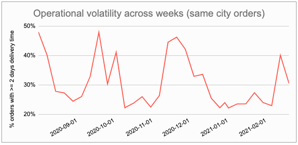
To compound the misery, COVID-19 added a large disruption with lockdown, manpower shortage etc.As an illustration of the operational volatility, below is a chart that shows the operational volatility for the same city orders at 1mg. We can see the percentage of orders taking 2 or more days to get delivered fluctuating between 25% and 50% week on week. On a regular day, this stays around 25% mark but then all of a sudden there is disruption. Inter city orders are even more prone to operational disruptions than the same city orders.

What didn’t work

To solve for the volatility in operations, the models needed to quickly capture the operational scenarios and be very agile in adapting to the ever changing scenarios. This section covers some of the things which we tried out but were not working. To read what worked directly, please feel free to skip this section.

1. Frequent retraining of models

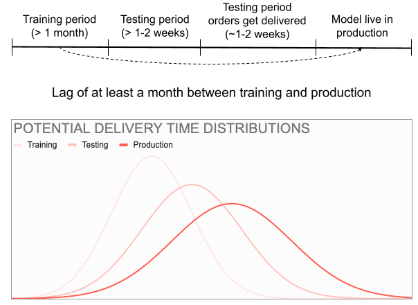
One of the solutions that we tried was retraining our models at a high frequency (daily/weekly) using recent data (last ~1 month). The idea behind this was simple. Just keep retraining on the latest data to keep the model updated and predict according to the latest scenario.However, the lag between training and production period ensured that this solution did not work. Assuming that the orders take 5 days on average to get delivered, there is a lag of at least a month between the training period to production due to: 1) Training period length (to get sufficient representative data for training),2) Testing period length at least a week3) Time for testing period orders to get deliveredIf the delivery time distributions change across weeks as shown in the chart below, the predictions in production (darkest) would be based on the distribution from training (lightest) and hence not effective.

2. Using features on delivery time of recently delivered orders

Another solution we tried was to capture the distribution changes by using the delivery time of recently delivered orders as features to the model. The idea here was to cut short the lags due to training and testing period and adapt according to relatively more recent data. However, some lag still remained largely due to the time needed for orders to get delivered.To understand this better, let us assume that an order takes 5 days to get delivered on average. If we are predicting the ETAs today, we’ll probably use orders which got delivered in previous week which in fact were placed a week prior to that. This creates a lag of at least 2 weeks in passage of information which in a lot of scenarios is very outdated.

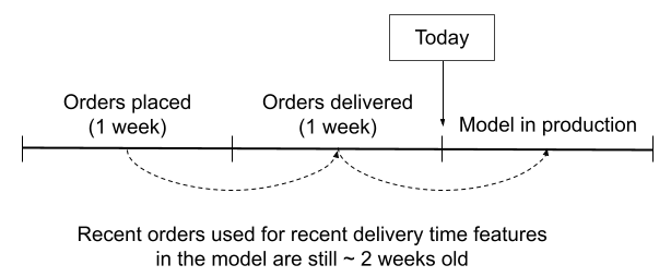Lag in using delivery time of recently delivered orders as a feature

3. Manually adding buffers

We also tried adding buffer time to the model’s prediction. This buffer time was suggested by the operations team based on the on ground knowledge they had, regarding the health of warehouses, delivery chain etc. For example, we added 1 day to all Mumbai orders because of monsoon rains (since last-mile delivery gets hit heavily).The key reason for this not working was that this insight was not always correct. It wasn’t a data driven buffer but more of a hunch of humans. Sometimes, the buffer would be applied too early or too late. Then there were cases where the severity of the issue could not be predicted.

How did we reach the ‘Eureka’ moment?

We made two major changes to our models which solved this volatility problem. One was to capture the real time health of operations through features on how different parts of the operations were performing. Second was on improving the ETA bucket definition. Let’s go into the depth of both of these.

1. Realtime indicator of operational health

To capture the operational health, we needed features which:

• Monitor the health of different parts of the entire order fulfilment chain
• Detect any abnormalities in any part and also gauge it’s extent
• Be as quick as possible in detecting any problems in operations
• Be agnostic of the cause of disruption if any

The queues for order fulfilment at 1mg are prescription verification, packaging, shipping and last mile delivery. We measured the status of operations for a particular queue through features capturing:1) The speed which orders are getting processed for the queue2) The backlog of orders waiting to be processed for the queue

This ensured that we were able to observe the happening and extent of any disruption in the entire chain as soon as it happened. If there is a disruption, whatever the cause maybe, it would be visible through this mechanism.

Operational health measurement for a simple scenario

Depending on the queue, the granularity of measurement was chosen. For example, the packaging queue was measured at the level of a warehouse. The delivery city or the delivery partner becomes irrelevant here. On the other hand, last mile delivery was measured at delivery city and delivery partner level. For last mile delivery the warehouse or the type of SKUs are irrelevant. Also, where ever applicable, we used separate features for separate type of orders (with different prioritization queues).

2. Variable ETA buckets with quantile loss function

Another self constructed constraint was a fixed bucket size. Generating an ETA window with a fixed bucket size is not appropriate when the underlying distribution is volatile. Even with accurate median prediction, an inappropriate bucket size fails the model with undesired level of breaches and early deliveries. For example, if the distribution is such that any 2 day window would yield a maximum of 50% accurate predictions, that’s the upper cap a model can achieve. Usually, when there is a disruption, we have observed the distribution to flatten; an increase in uncertainty or noise.

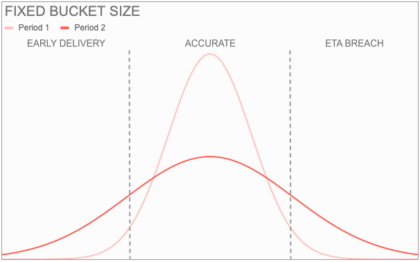
A variable bucket size works well with volatile distributions. With variable bucket size, the bucket size changes according to the scenario to ensure the desired level of accuracy. When the underlying distribution is more spread out (flat), a wider bucket is generated to ensure the same level of accurate prediction (and breaches & early deliveries). Whenever the distribution is such that any 2 day window would yield a maximum of 50% accurate predictions, the model automatically understands the increased uncertainty and increase the bucket size to attain the desired level of accuracy.

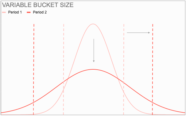
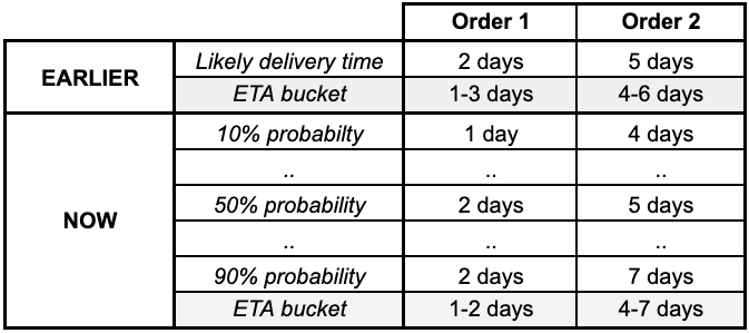
Apart from the bucket size, the method of generating this window was not optimal. We used the model prediction of most likely delivery time (median prediction) and created a window around it by adding and subtracting a day.We used quantile loss function to achieve both these things for ETA bucket definition. Quantile loss function enables the model to predict the target at different probability thresholds. We used it to generate different probable ETAs for a single order. For example, instead of just one prediction of 3 days, now our model predicts 10% chance of getting delivered in 2 days and 90% chance of getting delivered in 3 days. This enabled us to create an ETA bucket for each order based on the desired level of breach probability and early delivery probability.To help in better understanding, here is the change in our predictions for two hypothetical orders:

Evidence

With the above two major changes in our models, let’s see how they have been working.

Evidence 1: Week on week accuracy and breach for last 6 months

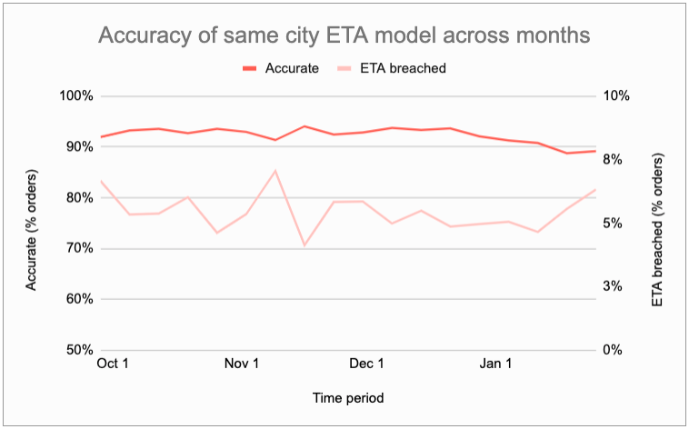
The accuracy for our models has been stable for months. As an example, below is a the accuracy and breach for our same city orders model. We can see the accuracy hovering in the 90%-95% range and breach around 5% mark.

Evidence 2: Testing period results from peak COVID-19 impacted period

These are the results from our testing period (not production results) for our same city ETA prediction model. Even during April 2020, when the operations were extremely disrupted with lockdown getting announced in many regions in the nation, the model shows decent accuracy level for most of the weeks. The 72% accuracy number may look low but to put things into context, this was a week when ~30% same city orders took 5 or more days to deliver; ~70% orders took 2 or more days (as compared to ~25% range we looked at the beginning of this article). Another point that can be seen here is that the breach percentages have remained the same from the testing period in May 2020 till date.

Evidence 3: Model adapting in two different operational scenariosAs a last evidence, we will look at a comparison of two scenarios: 1) Normal period in which operations were functioning smoothly, 2) Disrupted period in which the operations were facing challenges.First, let’s look at the delivery times during both these periods. As we can clearly see, during the disrupted period, orders took much longer to get delivered than the normal period.

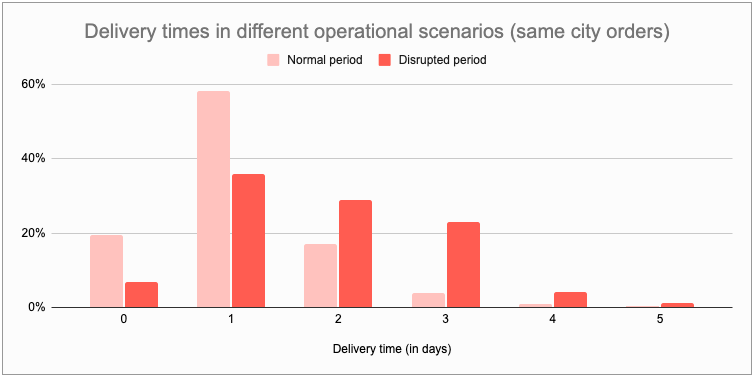
Now, let’s look at the our model’s ETA predictions during both these scenarios. Again, we can see clearly that model senses the change in operations and adjusts the ETA predictions to maintain low level of breaches.

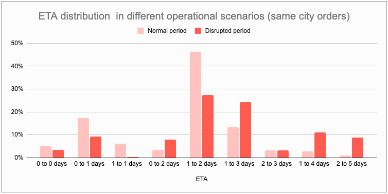
Finally, these are the performance metrics for both periods. Both are pretty indistinguishable in terms of these metrics. Guess yourself which one belongs to which period.

As a matter of fact, we ourselves aren’t able to notice operational disruptions by looking at the accuracy metrics these days. It’s only when we dig deeper and look at the delivery times, we find such scenarios. And this is how our game of whack-a-mole has come to an end.

A huge thanks to Rajat Chandiwala for working whole heartedly on the ETA problem. I would also like to thank Gaurav Agarwal, Kabir Soeny, PhD & Utkarsh Gupta for providing constant guidance and direction. And lastly, thank you Sneha for putting in so much effort to bring this article to the best shape.

Next Up: Managing wider ETA buckets

An arguable side effect of the above construct is wider ETA buckets during volatile operations since model captures the uncertainty and widens the bucket. This is a mathematically logical solution but wider ETA buckets are not good for the customers.To solve for the wider buckets, we have developed a framework which calculates revised ETA throughout the order’s lifecycle and enables revisions of ETA buckets in case of early deliveries, more precise ETA buckets or early detection of orders about to breach the ETA.We’ll talk about this framework in the next part of this series.Hit the 👏 button if you liked this article and share it with your friends. Also, share how you train your prediction model or if you have any feedback in the comment section below.

---

Predicting delivery time in volatile operational scenarios was originally published in Tata 1mg Engineering on Medium, where people are continuing the conversation by highlighting and responding to this story.